Bell’s theorem provides a way to discriminate between classical correlations and those obtained using quantum resources. The possibility of proving that certain correlations cannot be simulated classically is remarkable. However, is it possible to quantify the degree of deviation from classical behaviour? Can we conclude that one correlation is inherently more classical than another?
The set of correlations For an experiment under the no-signalling assumption (an experiment composed of different ‘locations’ which are assumed to be so well separated that it is impossible that a signal could have travelled between them) and with a fixed set of settings and outcomes, the set of classically realizable correlations is a strict subset of what can be achieved quantum mechanically. The following figure abstractly represents the set of no-signalling correlations, containing both the classical correlations and the set of the ones which are quantum-realizable. The set of classical behaviours and the set of no-signalling behaviours have ‘flat sides’, i.e., they are polytopes, and are convex: convexity in this case represent the fact that if we take the probabilistic mixture of two behaviours in one of these sets we’ll always remain in it. Note that the set of quantum-realizable empirical models is convex but not a polytope.
![]()
The typical characterisation of these sets in quantum foundations involves the notion of Bell inequalities. Bell’s theorem provided an inequality satisfied by all classical behaviours but violated by quantum correlations. Later, Bell’s derivation was simplified in the work of Clauser, Horne, Shimony, and Holt (CHSH). Following these seminal works, a plethora of different inequalities have been proposed. The idea is straightforward: no-signalling empirical behaviours can be described as vectors (the details of which are described in Stefano’s blog post), and inequalities for these correlations are defined as tuples $(a, R)$, where $a$ is a vector of the same dimension as the empirical models, and $R$ is a real bound.
These inequalities describe an affine hyperplane. For a model $e$, the inequality is satisfied whenever $e \cdot a \leq R$. They are considered tight if saturated by some non-classical and no-signalling correlations. The following figure represents the set of no-signalling correlations, to which we add a facet-defining inequality that separates the classical behaviour from a subset of the quantum correlations:
![]()
Quantifying Non-Classicality with Inequalities
A way to quantify non-classicality is to measure how much a given vector violates the bound specified by the inequality. For example, consider the CHSH inequality. This scenario involves two parties, each with two settings and two outcomes. Let us denote:
\[\text{CHSH} := E(A_1 B_1) + E(A_1 B_2) + E(A_2 B_1) - E(A_2 B_2),\]where $E(A_x B_y)$ is the expectation value of the correlation between measurements $A_x$ and $B_y$, calculated as follows:
\[E(A_x B_y) = p(00 | A_x B_y) + p(11 | A_x B_y) - p(01 | A_x B_y) - p(10 | A_x B_y)\]Clauser et al. observed that, for classical conditional distributions, we always have $\text{CHSH} \leq 2$. To check that this is in fact the case is straightforward, it is enough to probe the inequalities on the deterministic behaviours and appeal to the linearity of the expected values.
Classical distributions arise from no-signalling deterministic behaviours, obscured by the ignorance of some exogenous variables: mechanisms compatible with the ordinary notion of causality, where randomness only represents the presence of some exogenous factor in the model. In contrast, there exists no-signalling behaviour, such as the one known in the literature as the PR box, which not only violates the inequality but saturates it to the algebraic bound $\text{CHSH} = 4$. The behaviour of a PR box is described by the following table:
| $(0 0)$ | $(0 1)$ | $(1 0)$ | $(1 1)$ | |
|---|---|---|---|---|
| $(A_1 B_1)$ | $\dfrac{1}{2}$ | $0$ | $0$ | $\dfrac{1}{2}$ |
| $(A_1 B_2)$ | $\dfrac{1}{2}$ | $0$ | $0$ | $\dfrac{1}{2}$ |
| $(A_2 B_1)$ | $\dfrac{1}{2}$ | $0$ | $0$ | $\dfrac{1}{2}$ |
| $(A_2 B_2)$ | $0$ | $\dfrac{1}{2}$ | $\dfrac{1}{2}$ | $0$ |
In the PR box, the outputs are always correlated except when both agents choose the measurements $A_2$ and $B_2$.
The Tsirelson Bound and PR Box
For the PR box, the value of the CHSH inequality is $4$, the algebraic maximum. It can be shown that quantum mechanics cannot entail correlations which are that strong, but it can nevertheless violate the CHSH inequality by achieving a value of $2 \sqrt{2}$, known as the Tsirelson bound. This is the maximum attainable with quantum resources in the two-setting, two-outcomes scenario. The PR box, although unachievable with quantum resources, represents a behaviour that is more non-classical than anything attainable with quantum systems.
The extent to which a conditional probability distribution violates a Bell inequality cannot alone certify its degree of non-locality. In particular, a given inequality may not be violated by certain non-classical correlations. While a violation suffices to prove non-classicality, it is generally far from necessary.
There are two problems with such inequalities. The first is that a single inequality may not be enough to detect the non-local content of all behaviours for a given scenario. For example, relabelling $A_1$ with $A_2$ gives a CHSH inequality that is not violated by the PR box we have described earlier. In fact, in this case, the inequality:
\[E(A_2 B_1) + E(A_2 B_2) + E(A_1 B_1) - E(A_1 B_2) \leq 2\]is satisfied by our non-classical behaviour despite being tight, this is because it refers to a different facet of the polytope! The following figure can help us provide an intuition:
![]()
The second problem is that the deviation from the bound $R$ needs to be renormalized to allow a homogeneous discussion of non-classicality, which may have different meanings across different inequalities. The normalized violation of the inequality $(a,R)$ for an empirical model $e$ is:
\[v_{a,R}(e) := \dfrac{\max{\left (0,a \cdot e - R \right)}}{\lVert a \rVert -R}.\]In this equation, $\lVert a \rVert$ is the maximal algebraic violation. When we calculate $v_{a,R}(e_{PR})$ for the vector associated to the empirical model of the PR box, we achieve a violation of $1$, while anything classical, for which $a \cdot e - R \leq 0$, is evaluated to $0$. We should be careful about the fact that a single inequality captures at most (when tight) the structure of a single facet of the classical polytope:
![]()
The Local Fraction
An alternative approach to quantifying non-locality is by appealing to the local fraction, which directly answers the question: what is the largest part of an empirical model that can be simulated by classical resources? Formally, we seek a decomposition of $e$:
\[e = \epsilon e_L + (1 - \epsilon) e_N\]where $\epsilon$ is the local fraction, and $e_L$ is a local, classical behavior. The local fraction $\epsilon$ can be understood as the maximal fraction of the model that can be recovered by only making use of classical resources. Abramsky et al. showed that $1 - \epsilon$ provides an upper bound to any Bell inequality violation. Moreover, there always exists an inequality for which the normalized violation equals $1 - \epsilon$.
This quantity can be calculated by solving a linear system of equations as described in more detail in this blog post on Bell’s theorem. There is no need to understand the facets defining inequalities; it is only important to understand the deterministic behaviours compatible with a given scenario (this is why the approach is particularly suitable for the study of non-locality under arbitrary causal assumptions, e.g., see arxiv.org/abs/2403.15331).
By using linear programming, we can calculate the maximal local fraction (that can be achieved by allowing two choices of equatorial projective measurements) as a function of the two angles used. What emerges is a landscape of values that changes as a function of the chosen angles $(\phi_0,\phi_1)\in[0,\pi]\times[0,\pi]$:
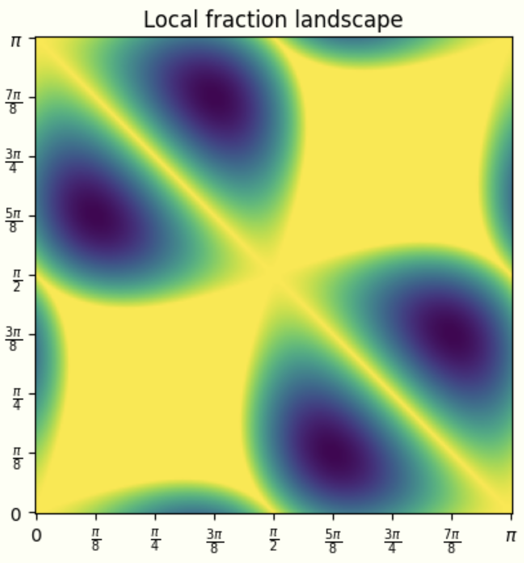
We see deep blue valleys, which represent where the local fraction is minimal, and yellow plateaus, where the correlations can be entirely classically simulable. The minimum local fraction for these equatorial measurements is approximately $0.5858$ and there is a correspondence to the Tsirelson bound: this can be shown substituting $R = 2$ and $\lVert a \rVert$, $e - R = 2\sqrt{2}$ into the formula for the normalized violation of Bell’s inequalities:
\[\dfrac{\max{\left (0,a \cdot e - R \right)}}{\lVert a \rVert - R} = \dfrac{2\sqrt{2} - 2}{4 - 2} = \sqrt{2} - 1\]which is approximately $1 - 0.5858$, the maximal local fraction for equatorial measurements.
Increasing the Number of Settings
The local fraction in the figure above has been calculated under the assumption that there are two parties sharing a maximally entangled resource and that they always interact with it by choosing between two projective measurements. What happens when we increase the number of available settings per agent?
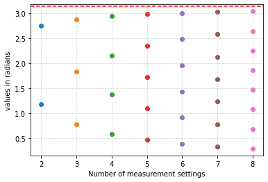
Suppose, for example, that Alice and Bob now choose between three angles on the XY plane of the Bloch sphere. These angles all represent different projective measurements, and we can now calculate the minimal local fraction using linear programming in conjunction with optimization techniques like COBYLA to find the optimal angles for the measurement settings. COBYLA is an optimization algorithm that can be used to find the best solution to a problem with constraints. A peculiarity of the algorithm is that it performs the optimization without knowing anything about how much a small change influences the outcome, i.e., without having knowledge of its derivative. We already know that the optimal angles for two settings are given by $\left[\frac{\pi}{8}, \frac{5\pi}{8}\right]$. For three settings, the optimal angles are $\left[\frac{\pi}{12}, \frac{5\pi}{12}, \frac{7\pi}{12}\right]$, and for four: $\left[\frac{\pi}{16}, \frac{5\pi}{16}, \frac{9\pi}{16}, \frac{13\pi}{16}\right]$. We can plot the angles on Bloch spheres for better visualization:
As the number of angles increases, the local fraction converges rapidly to $0$, enabling us to extract higher degrees of non-classicality. In the following picture we showcase the angles that we have calculated for the number of settings ranging from $3$ to $8$ (the dashed red line represents $\pi$, these are all angles from $0$ to $\pi$ parametrising the equatorial measurements).
For eight angles, the local fraction drops below $0.16$. To visualize the trend that this diminishing degree of classicality entails, we can plot the local fraction as a function of the number of settings:
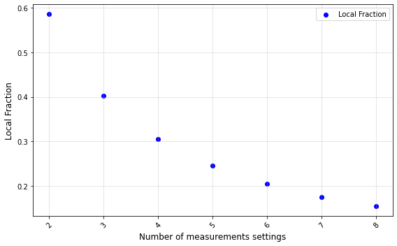
Increasing the number of settings significantly lowers the fraction of the behaviour that is classically simulable. We can extract as much non-classicality as we wish from a single shared entangled state!
The following interactive simulation provides a visual representation of the local fraction for cases where the agents can choose between three different angles. The result is a plot similar to the one our readers may be familiar with, but in three dimensions. As usual, the colours of the dots represent the degree of non-classicality obtained by the model for a given choice of angles, $(\theta_1, \theta_2, \theta_3)$. Readers who wish to explore the figure can use it to navigate towards one of the twelve minima. This multiplicity arises because the three angles can be permuted in 6 ways, combined with symmetries from considering supplementary angles (e.g., replacing all $\theta$ with $\pi − \theta$), doubling the solutions.
These findings suggest that the Tsirelson bound is an artefact of the chosen experimental setup. By expanding the set of measurement settings, a pair of entangled qubits can witness arbitrarily high non-locality. Any bound on non-locality arises from the constraints imposed by the classical interface used to access quantum systems, rather than being an inherent limit to the production of non-local correlations.
Why is this important? The impossibility of simulating, in principle, some behaviours using classical resources is a fundamental factor in the development of device-independent cryptographic protocols. The existing protocols usually rely on the violation of certain inequalities and are typically bound to the two-settings and two-outcomes scenario.
In a 2006 paper by Stephanie Wehner, she studies generalized Tsirelson bounds for a broader class of CHSH inequalities:
\[\left|\sum_{i=1}^n E(A_i B_i)+\sum_{i=1}^{n-1}E(A_{i+1}B_i)-E(A_1B_n)\right| \leq 2n-2\]These inequalities bound the polytope of classical behaviours with multiple settings and binary outputs and have been shown by Froissart and Tsirelson to correspond to the faces of the polytope of classical behaviours with $n$ settings. Stephanie Wehner proves that while quantum mechanics violates the generalized CHSH inequalities, it still satisfies the following bound:
\[\left| \sum^n_{i=1}E(A_iB_i) + \sum_{i=1}^{n-1}E(A_{i+1}B_i)-E(A_1B_n)\right|\leq 2n\cos\left(\dfrac{\pi}{2n}\right)\]Specifically, she proves using semidefinite programming that there exist quantum mechanical setups that saturate this bound. Since the generalized CHSH inequalities fully characterize the structure of the polytope, it should be possible to compare these analytical results with the local fraction obtained by finding the optimal angles through our optimization techniques. To do so, we renormalize the maximal quantum violations obtained by Stephanie Wehner: in this case, $R = 2n-2$, the maximal algebraic violation is $2n$, and the maximal quantum violation is $a \cdot e = 2n\cos\left(\dfrac{\pi}{2n}\right)$:
\[\dfrac{\max{\left (0,a \cdot e - R \right)}}{\lVert a \rVert -R} = \dfrac{2n\cos\left(\dfrac{\pi}{2n}\right) - 2n +2 }{2} = n(\cos\left(\dfrac{\pi}{2n}\right) -1) + 1\]Thus, the local fraction is $n\left(1-\cos\left(\dfrac{\pi}{2n}\right)\right)$, which agrees perfectly with our numerical results.
If the notion of the Tsirelson bound can be generalized to certain scenarios, it ceases to be equally meaningful when, for example, we change the number of outputs or modify the causal structure of the protocol. The analytical technique would be powerless, but our numerical exploration would continue to provide useful insights. By now, the reader should be convinced that there is no need to construct complex inequalities to characterize the facets of these high-dimensional polytopes. The local fraction, with its homogenizing power, simplifies the accounts of non-locality. We believe that pinpointing the correct mathematical formulation of non-locality is essential for correctly understanding and harnessing the great power bestowed by non-local correlations. This research is still in its infancy, and there is much more to explore—stay tuned!