In this post, we provide a brief introduction to Bell’s Theorem, a landmark mathematical result proving that the statistics observed in quantum mechanical experiments are incompatible with a local hidden-variable description.
Bell’s Theorem is often stated as the violation of a CHSH inequality, but there are several alternative formulations which can be used to conclude the same incompatibility. Here, we discuss the result from an operational perspective, focusing on actions which can be performed and outcomes which can be observed as part of a repeatable experiment, with limited to no assumptions on the underlying physics. This is the fundamental, protocol-oriented philosophy behind contextual cryptography.
Bell Test
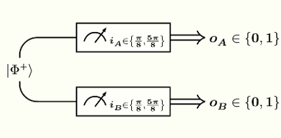
Two parties — call them Alice and Bob — each have one of two qubits in an entangled state $\vert\Phi^+\rangle$, as shown by the following circuit:

The state $\vert\Phi^+\rangle$ can be expanded as follows in the computational basis:
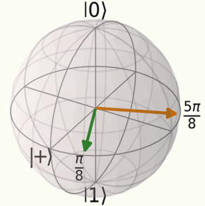
\[\vert\Phi^+\rangle = \frac{\vert 00 \rangle+\vert 11 \rangle}{\sqrt{2}}\]Alice and Bob are free to measure their qubits in one of two possible bases, defined by axes at angles of $\frac{\pi}{8}$ and $\frac{5\pi}{8}$ from the $\vert+\rangle$ state along the Bloch sphere’s equator:

The quantum state $\vert \psi_{\theta} \rangle$ at an angle $\theta$ from $\vert+\rangle$ can be expanded as follows in the computational basis:
\[\vert \psi_{\theta} \rangle = \frac{\vert 0 \rangle + e^{i\theta} \vert 1 \rangle}{\sqrt{2}}\]The inputs for this experiment are the measurement choices: they are binary, taking values $i_A, i_B \in \lbrace 0, 1 \rbrace$ by convention, but it is more convenient to directly work with the corresponding measurement angles $\theta_A, \theta_B \in \lbrace\frac{\pi}{8}, \frac{5\pi}{8}\rbrace$:
\[\theta_X = \frac{\pi}{8}+i_X\frac{\pi}{2} \text{ for } X = A, B\]Alice and Bob measure their qubits simultaneously, by selecting their inputs randomly and free of any constraints. The outputs for this experiment are the measurement outcomes: they are also binary, taking values $o_A, o_B \in \lbrace 0, 1\rbrace$ by convention. This kind of experiment is known as a Bell test.
Note that simultaneity of measurement is not strictly necessary: it is enough to somehow enforce the no-signalling condition, i.e. to ensure that no communication is possible between the measurement devices from the moment the input is selected to the moment the output is displayed and recorded. Simultaneity provides a way to derive the no-signalling condition from the laws of relativistic physics, but simpler approaches based on concrete setup considerations can be used in practice.
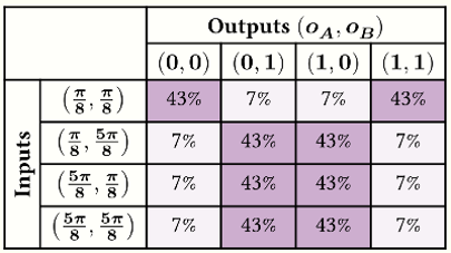
Alice and Bob repeat the experiment for many rounds, recording the observed input-output pairs, and then meet to compute joint statistics. The following table shows the resulting (approximate) probability distribution for the four possible joint output pairs $(o_A, o_B)$, conditional to the four possible joint input pairs $(\theta_A, \theta_B)$, in the ideal case where the experiment is performed without any noise and in the limit of a large number of rounds:

We can explicitly compute the probabilities in the table above using the Born rule, together with the computational basis expansions previously listed for the states involved:
\[\begin{aligned} &P\left(o_A, o_B\,\middle\vert\, \theta_A, \theta_B \right) \\ =& \left\vert \left( \langle \psi_{\theta_A\,+\,o_A\,\pi} \vert \otimes \langle \psi_{\theta_B\,+\,o_B\,\pi} \vert \right) \vert\Phi^+\rangle \right\vert^2 \\ =& \frac{1}{8} \left\vert 1+(-1)^{o_A \oplus o_B}\;e^{-i(\theta_A+\theta_B)} \right\vert^2 \\ =& \frac{1}{4} \left( 1+(-1)^{o_A \oplus o_B}\cos\left(\theta_A+\theta_B\right) \right) \end{aligned}\]By substituting the labels of the table rows and columns for $(\theta_A, \theta_B)$ and $(o_A, o_B)$, respectively, we obtain the specific probability values shown above.
Hidden-Variable Models
The fundamental physical question which Bell’s Theorem contributes to address is whether the randomness observed by Alice and Bob is intrinsic, or whether instead it could be pre-determined with sufficient knowledge of the physical conditions around the experiment. Originally of interest for philosophical reasons, as part of a long-standing dispute about the interpretation of quantum theory originating from the 1935 EPR paper, this question has fundamental implications for cryptography, where the impossibility to for attackers to predict observed randomness is directly linked to security.
The hypothetical knowledge assumed for the purposes of pre-determinability can include, for example, the exact contents of the experimental devices, as well as the exact setup of the labs and everything which surrounds them. However, it is important that we don’t presume any knowledge about the inputs $\theta_A, \theta_B$, which must remain (approximately) uniformly random. For foundational purposes, a common assumption in this regard is that the inputs are chosen by Alice and Bob themselves, and that the content of their minds is excluded from the realm of knowable information for the purposes of the pre-determination question. Cryptographically, a better assumption is to presume that the random inputs are produced by local secure random number generators, resulting in a possible characterisation of contextual cryptographic protocols as ways to transform secure local randomness into secure shared randomness.
In its simplest form, the question of pre-determinability of the observed randomness could be mathematically formalised as follows: Could there be some hidden variable $\mathfrak{L}$ — a random variable unknown to Alice and Bob, and independent of the input choices, but potentially known to an attacker and correlated with the experimental outcomes — such that conditioning to a definite value $\lambda$ for $\mathfrak{L}$ renders the experimental probability distribution fully deterministic?
\[\begin{aligned} \mathbb{P}\left(\underline{o}\,\middle\vert\, \underline{\theta} \right) &= \sum_{\lambda} \mathbb{P}\left(\underline{o}\,\middle\vert\, \underline{\theta}, \lambda\right) \mathbb{P}\left(\lambda\right) \\ \mathbb{P}\left(\underline{o}\,\middle\vert\, \underline{\theta}, \lambda \right) &\in \lbrace 0, 1\rbrace \end{aligned}\]The hidden variable $\mathfrak{L}$ in this definition could be almost anything, and we’ve kept our probabilistic notation vague on purpose. In an effort to make things more precise, we consider the following equivalent formulation of our question: Can we define a function $F$ mapping a joint input choice $\underline{\theta} = (\theta_A, \theta_B)$ together with a value $\lambda$ of the hidden variable to a single deterministic output pair $\underline{o} = (o_A, o_B)$ for the experiment?
\[\mathbb{P}\left(\underline{o}\,\middle\vert\, \underline{\theta}, \lambda \right) = \begin{cases} 1 & \text{ if } \underline{o} = F(\underline{\theta}, \lambda)\\ 0 & \text{ otherwise} \end{cases}\]This second formulation is more explicit, and it hints at a possible role played by functions in the definition of hidden-variable models. To pursue this intuition, we consider set of all $(2^2)^{(2^2)} = 256$ possible functions mapping joint inputs to joint outputs for our experiment as well as any other experiment with the same “shape”:
\[\left\lbrace \frac{\pi}{8}, \frac{5\pi}{8} \right\rbrace^2 \rightarrow \lbrace 0, 1 \rbrace^2\]We observe that, for any fixed value $\lambda$ of the hidden variable, the partial evaluation $F(\underline{}, \lambda)$ is one of these 256 functions. We also observe that any two distinct values $\lambda \neq \lambda’$ of the hidden variable resulting in the same $F(\underline{}, \lambda) = F(\underline{}, \lambda’)$ are operationally indistinguishable.
Following the observations above, we arrive at a final, combinatorially explicit formulation of our question: Can we define a probability distribution $H$ on the set of functions above such that the probability on joint outputs for each given joint input coincides with that observed in the experiment?
\[P\left(\underline{o}\,\middle\vert\, \underline{\theta} \right) \hspace{3mm} = \hspace{-8mm} \sum_{\substack{ f: \left\lbrace \frac{\pi}{8}, \frac{5\pi}{8} \right\rbrace^2 \rightarrow \lbrace 0, 1 \rbrace^2 \\ \text{s.t. }\; \underline{o} \;=\; f(\underline{\theta}) }} \hspace{-8mm} H(f)\]We refer to such a probability distribution $H$ as a hidden-variable model:
\[H \in \mathcal{D}\left( \left\lbrace \frac{\pi}{8}, \frac{5\pi}{8} \right\rbrace^2 \rightarrow \lbrace 0, 1 \rbrace^2 \right)\]This is an abstract, implementation-independent description to which every hidden variable can be reduced:
\[H(f) := \hspace{-4mm} \sum_{\substack{\lambda \text{ s.t. } \\ F(\underline{}, \lambda) = f}} \hspace{-3mm} \mathbb{P}(\lambda)\]Simple as it may be, this definition of a hidden-variable model doesn’t actually help to address our question: one such model always exists. Indeed, it is easy to show that the conditional probability distributions for fixed input and output sets form a convex polytope, with the deterministic distributions — those valued in $\lbrace 0, 1 \rbrace$, corresponding to the 256 functions — as the vertices of the polytope. This polytope is not generally a simplex, so there can be many hidden-variable models $H$ which reproduce the same conditional probability distribution $P$, but we are guaranteed that one such $H$ always exists.
Just as centuries worth of classical physicists and philosophers before us, we might at this point be tempted to conclude that all experimentally observed randomness can be pre-determined, the only limitation being our imperfect practical knowledge of the physical processes which govern the universe around us.
We would be wrong.
Local Hidden-Variable Models
It is a mathematical fact that hidden-variable models exist for any conditional probability distribution. For such a hidden-variable description to be physically meaningful, however, it is not enough that it reproduces the observed statistics: it must do so consistently with any additional constraints imposed on the experiment, either by us or by Physics.
At the very least, hidden-variable models should respect the signalling restrictions imposed by the causal structure of spacetime: information cannot travel faster than the speed of light. This is known as the principle of locality, or the no-signalling principle, and hidden-variable models respecting it are known in the literature as local hidden-variable models.
Concretely, a local hidden-variable model — sometimes styled as LHVM — is a hidden-variable model $H$ which is entirely supported by functions which respect the no-signalling principle, i.e. those where Alice’s output cannot depend on Bob’s input and Bob’s output cannot depend on Alice’s input:
\[H(f) > 0 \Rightarrow \begin{cases} f(\underline{}, \frac{\pi}{8})_A = f(\underline{}, \frac{5\pi}{8})_A \\ f(\frac{\pi}{8}, \underline{})_B = f(\frac{5\pi}{8}, \underline{})_B \end{cases}\]Above, we have indicated Alice’s output by $f(\theta_A, \theta_B)_A$ and Bob’s output by $f(\theta_A, \theta_B)_B$. Equivalently, the functions $f$ satisfying the no-signalling principle in this scenario are those which factorise as $f = f_A \times f_B$, for a pair of functions $f_A$ and $f_B$ which determine the local input-output relationship for Alice and Bob, respectively:
\[f(\theta_A, \theta_B) = \left(f_A(\theta_A), f_B(\theta_B)\right)\]We have thus restricted ourselves to a subset of $2^2 \times 2^2 = 16$ no-signalling functions amongst our original set of 256: the conditional probability distributions which admit a local hidden-variable model lie in the polytope spanned by the corresponding subset of vertices. Finally, we can adequately formulate our original question about pre-determinability of randomness: Does the conditional probability distribution inferred from our experiment admit a local hidden-variable model?
The answer, as it turns out, is no: the randomness we observe in this experiment is, at least in part, intrinsic.
Non-local Fraction
To prove that the conditional probability distribution $P$ obtained from Bell’s Experiment does not admit a local hidden-variable model $H$, we start by observing that one such model can be constructed by solving a system of 16 equations (corresponding to the entries of the table for $P$) in 16 unknowns (corresponding to the probabilities of the 16 no-signalling functions $f = f_A \times f_B$):
\[P\left(\underline{o}\,\middle\vert\, \underline{\theta} \right) = \hspace{-8mm} \sum_{\substack{ f_A, f_B\,:\, \left\lbrace \frac{\pi}{8}, \frac{5\pi}{8} \right\rbrace \rightarrow \lbrace 0, 1 \rbrace \\ \text{s.t. }\; o_A \;=\; f_A(\theta_A) \\ \text{and }\; o_B \;=\; f_B(\theta_B) }} \hspace{-8mm} H(f_A \times f_B)\]For convenience, we use the RHS of the equation above to define the conditional probability distribution $P_H$ arising from any given local hidden-variable model $H$:
\[P_H\left(\underline{o}\,\middle\vert\, \underline{\theta} \right) := \hspace{-8mm} \sum_{\substack{ f_A, f_B\,:\, \left\lbrace \frac{\pi}{8}, \frac{5\pi}{8} \right\rbrace \rightarrow \lbrace 0, 1 \rbrace \\ \text{s.t. }\; o_A \;=\; f_A(\theta_A) \\ \text{and }\; o_B \;=\; f_B(\theta_B) }} \hspace{-8mm} H(f_A \times f_B)\]Using this, our question can be more neatly formulated as:
\[\exists H \text{ LHVM s.t.}\, P\left(\underline{o}\,\middle\vert\, \underline{\theta} \right) = P_H\left(\underline{o}\,\middle\vert\, \underline{\theta} \right)\]Additionally, the values of our 16 unknowns must be constrained to be non-negative, in order for $H$ to be a probability distribution:
\[H(f_A \times f_B) \geq 0 \text{ for all } f_A, f_B\]This suggests that what we are interested in is, in fact, the solution to a linear optimisation problem. Indeed, we can generalise our initial yes/no question (Does a local hidden-variable model $H$ exist which explains $P$?) to a broader quantitative question: What fraction of $P$ can be explained by some local hidden-variable model $H$? Or, more precisely: What is the maximum $\varepsilon_H \in [0, 1]$ such that the conditional probability distribution can be written as follows for some local hidden-variable model $H$ and some “remainder” conditional probability distribution $R_H$?
\[P = \varepsilon_H P_H + (1-\varepsilon_H) R_H\]Note that convex combinations of conditional probability distributions are taken componentwise, so that the succinct equation above can be expanded into the below:
Also, note that a suitable conditional distribution $R_H$ exists exactly when $\varepsilon_H P_H \leq P$ holds componentwise, and that it is furthermore unique whenever $\varepsilon_H < 1$:
\[R_H\left(\underline{o}\,\middle\vert\, \underline{\theta} \right) = \frac{ P\left(\underline{o}\,\middle\vert\, \underline{\theta} \right) - \varepsilon_H P_H \left(\underline{o}\,\middle\vert\, \underline{\theta} \right) }{1-\varepsilon_H}\]We define the local fraction for the conditional probability distribution $P$ to be the maximum possible such $\varepsilon_H$ over all local hidden-variable models $H$:
\[\max_{H \text{ LHVM}} \left\{ \varepsilon_H \,\middle |\, \varepsilon_H P_H \leq P \right\}\]The answer to the original yes/no question corresponds to the case where the local fraction is 1, in which case 100% of $P$ can be explained by a local hidden-variable model.
In order to compute the local fraction, we formulate a linear optimisation problem in standard form. We start by linearising the tables for $P$ and for the individual no-signalling functions — or, to be precise, for the corresponding deterministic conditional probability distributions. Below is the linearisation of the table for $P$, which will provide the constant vector for the linear inequalities in the problem:
As another example, below is the linearisation of the table for the function where the outputs of both Alice and Bob are fixed to 0 independently of their input:
We have fixed a total ordering $f_1,…,f_{16}$ of the no-signalling functions, and we write $\underline{h} \in \mathbb{R}^{16}$ for the vector corresponding to $\varepsilon_H H$ linearised with that ordering:
\[\underline{h} = \left(\begin{array}{c} H(f_1) \\ \vdots \\ H(f_{16}) \end{array}\right)\]The linear problem then consists of maximising the sum of the entries in $\underline{h}$, subject to the positivity requirement $\underline{h} \geq 0$ and the following upper-bound inequalities:
The 16 no-signalling functions $f_1,…,f_{16}$ correspond to the columns of the matrix above, with $f_1$ being the example shown earlier.
We can feed the linear problem to SciPy’s linprog, and we obtain a local fraction of ~58.58% for this experiment.
In other words, ~41.42% of the correlated randomness observed by Alice and Bob cannot be pre-determined (subject to enforcement of the no-signalling condition and randomness of their local input choices).
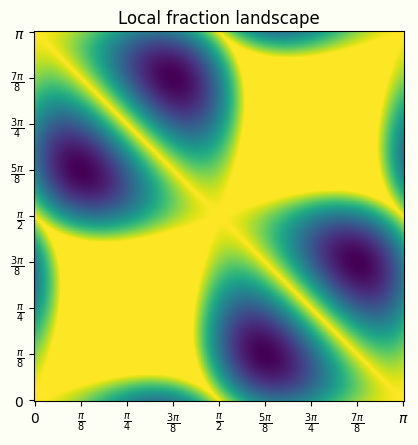
The specific angles $\frac{\pi}{8}$ and $\frac{5\pi}{8}$ used in our experiment were chosen to minimise the local fraction, i.e. to maximise the amount of randomness available for secure cryptographic purposes. To verify that this is truly the case, we can plot the local fraction for arbitrary choices of these two angles, reproducing the results of arXiv:1705.07918:

The bright yellow plateaus and ridges are the regions where the local fraction is 100%, i.e. where the randomness is fully explained by a local hidden-variable model, while the darker green/blue valleys are the regions where the non-local fraction is lower than 100%. The landscape is periodic by $\pi$ in the horizontal and vertical directions, and is symmetric about the diagonal and antidiagonal axes. The local fraction minima, the angles where the most randomness is intrinsic, are at the dark blue bottoms of those valleys, at point $\left(\frac{\pi}{8}, \frac{5\pi}{8}\right)$ and its 3 symmetric counterparts.
A Jupyter notebook with code for local fraction calculation can be found in this gist.